
About a year before I retired from MathWorks, I gave a presentation to the Image Processing Team called:
An Incomplete and Possibly True History of Image Display in MATLAB
Or: What’s Up with IMAGE and IMSHOW and IMTOOL and IMVIEW and …"
I thought some Harmonic Notes readers might be interested in this material. Some readers are MathWorks developers who want to know how various MATLAB features and behaviors came to be the way they are. Other experienced MATLAB users have told me that they are also curious to hear about MATLAB evolution.
I can tell a lot of the story from my personal experience and memory. I started using MATLAB in the late 1980s, and later I worked in MathWorks software development from 1993 to 2024. During much of my time at MathWorks, I was either leading or working closely with the Image Processing Toolbox development team. Some important changes happened during the years when I was concentrating more on MATLAB design, but I’ll do my best to fill in what I know about that time.
Before MATLAB
Digital imagery got started in the 1920s, with the transmission of images via oceanic cable across the Atlantic for newspaper publication. Computer-based image processing, including early image enhancement and restoration techniques, got started in the 1960s, especially with the work of the Jet Propulsion Laboratory on images transmitted by space probes.
A 1972 special issue of Proceedings of the IEEE featured the early research in two key areas: image compression and image restoration. A third key area took off in the 1970s with the invention of computed axial tomography, popularly known as the CAT scan. For more on the early history of digital image processing, see Gonzalez and Woods, Digital Image Processing, 4th ed., Pearson Education, 2018.
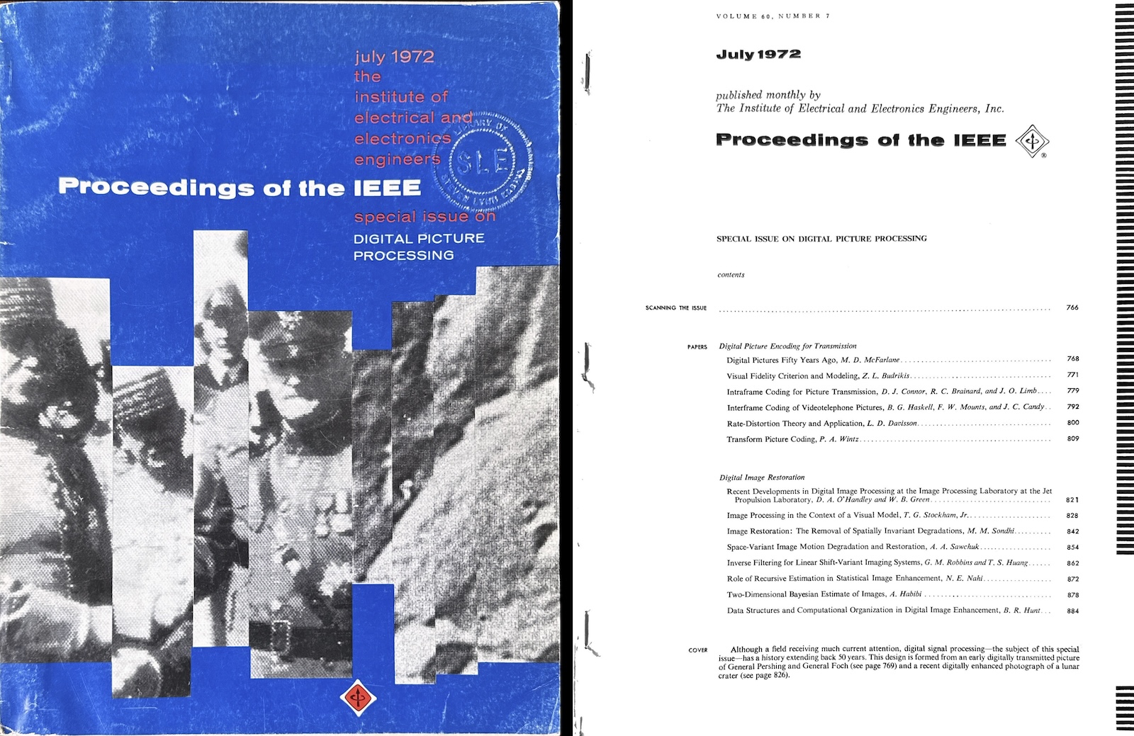
1972 Proceedings of the IEEE Special Issue on Digital Picture Processing, cover and table of contents
Late 1970s and Early 1980s
Cleve Moler’s original MATLAB, written in Fortran and distributed freely to university professors and researchers, had only primitive graphics display. Even line plots were rendered using text characters.
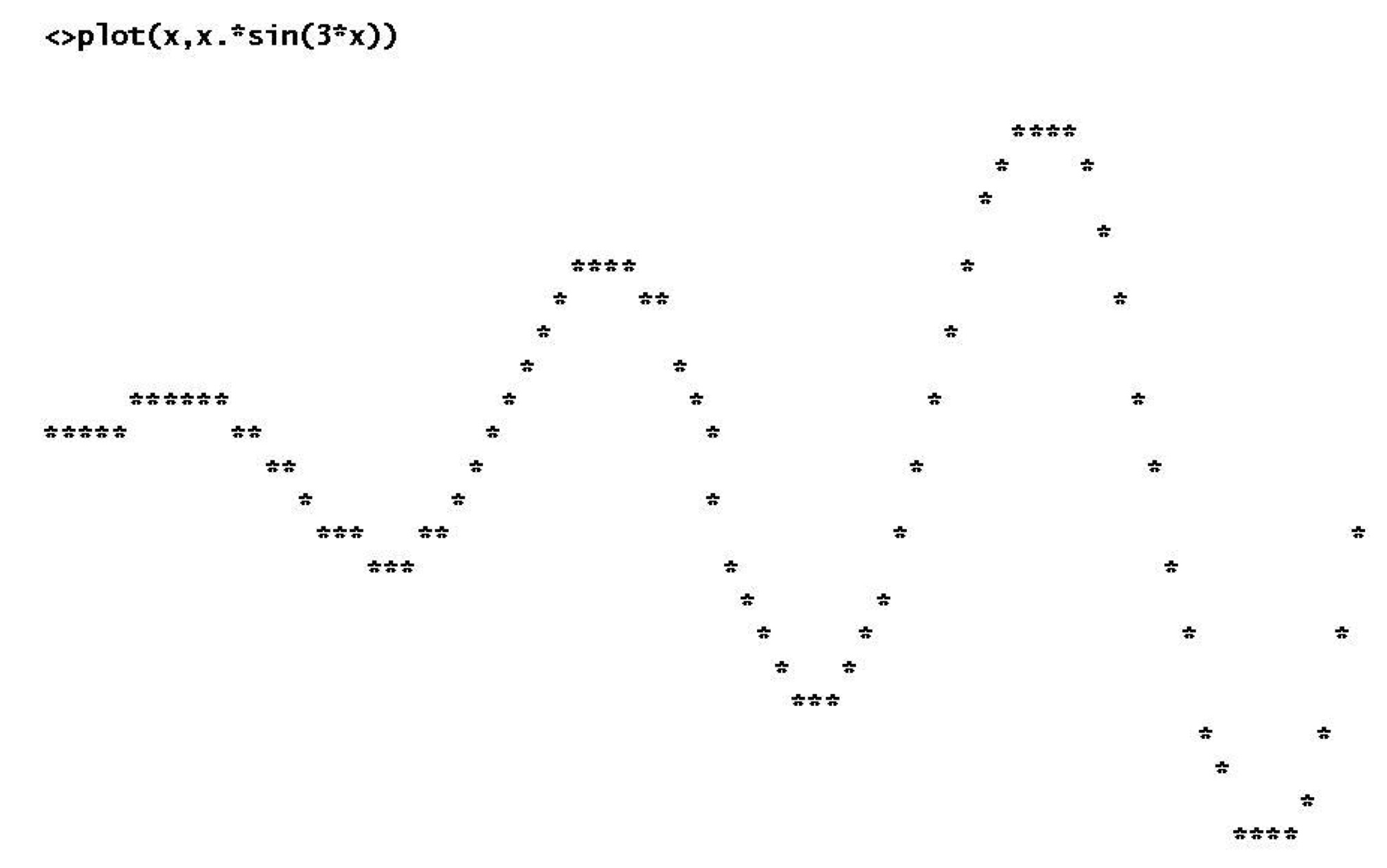
Character graphics in the late 1970s / early 1980s Fortran-based MATLAB. Source: “Evolution of MATLAB,” Cleve Moler
The first MathWorks release of the commercial version of MATLAB, on the PC, came in 1984. I do not have sample graphics from that version, but even rudimentary image display in MATLAB was still several years away.
Late 1980s
MATLAB version 3.0, followed by several point releases, arrived in the late 1980s. I bought this version of MATLAB while I was in graduate school at Georgia Tech. Here are some sample graphics from MATLAB 3, which did not support image display—at least, not officially.
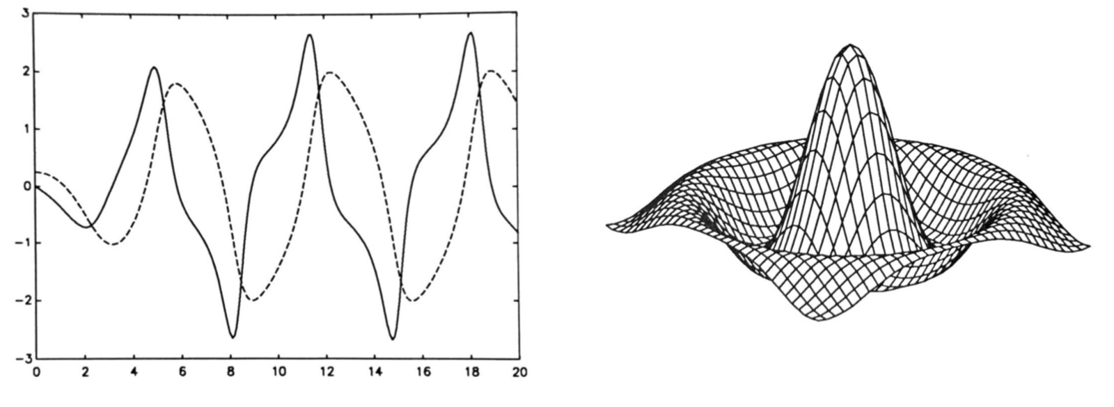
Sample graphics from MATLAB 3. Source: MATLAB for MS-DOS Personal Computers User’s Guide
At this time, it was becoming easier to do academic research in digital image processing. At Georgia Tech, where I was in grad school, the Digital Signal Processing research lab acquired a couple of Sun Workstations (initially Sun 3, and later a Sun Sparcstation). These had large, high resolution (for the time) monitors that could display images, and they ran Unix and the X Window System, or X11. Students doing image processing research used these workstations and typically programmed in Fortran or C.
It was still not possible to do significant image processing work in MATLAB then. Image display was not natively supported, and individual MATLAB variables were limited to 8,188 elements—about 90x90!
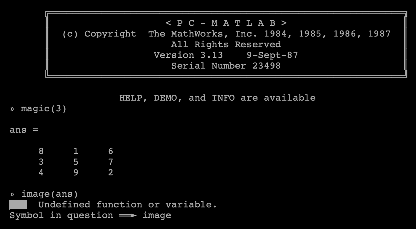
Screen shot from my MATLAB 3.13 running on a virtual DOS machine. As you can see, it has no IMAGE function.
I did hear, however, that a few people were beginning to experiment with it. MATLAB 3’s “MEX-file” support allowed users to create new MATLAB functions based on C or Fortran code, and some users created MEX functions for displaying images. I never tried this myself.
The image processing era in MATLAB had to wait until the arrival of MATLAB 4. That’s where I’ll pick up the story next time.