
Today’s post, the third in this series on the history of image display in MATLAB, describes the scene in 1993, when Image Processing Toolbox and the function imshow were released for the first time.

My 1993
In 1993, I was on the faculty of the Electrical Engineering and Computer Science department at the University of Illinois at Chicago. The UIC job wasn’t working out well for me, and so I was looking for new job. I searched for another faculty position at first, but then I started thinking about MathWorks and MATLAB. I used MATLAB extensively, and I was impressed with the MathWorks engineers and developers.
I met Loren Shure, the first MathWorks hired employee, at ICASSP in Minneapolis in April, and later I sent her my resume. After she graciously informed me that there were no suitable job openings, I reminded her that I had volunteered to beta test the Image Processing Toolbox, and she added me to the beta list.
I treated the beta test program as a job audition opportunity. I spent much of the summer studying the toolbox in depth, and I provided numerous enhancement suggestions, bug reports and fixes, performance improvements, and demo ideas.
Here is a small portion of the beta survey form that I completed. Notice how I focused on image display issues. I’ll come back to that later.
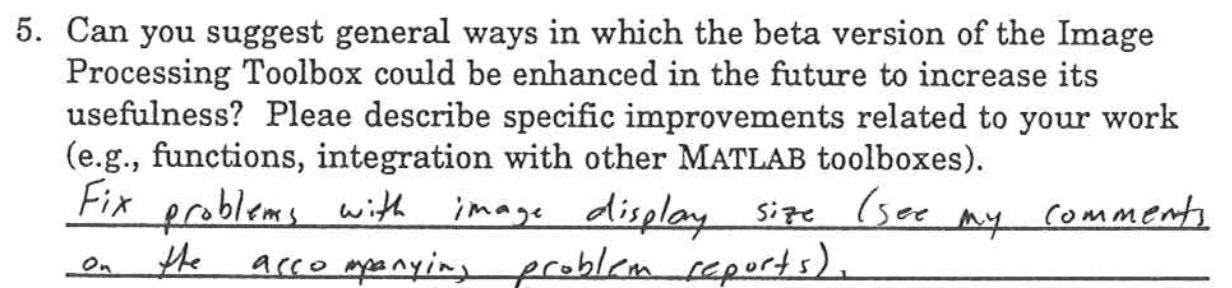
Excerpt from Steve Eddins beta survey form, Image Processing Toolbox version 1.0 beta, 1993
After the beta test program wrapped up, I was invited to interview with MathWorks in September. During the afternoon of my interview day, I brainstormed a product demo idea with Loren and Clay Thompson; my sketches on Clay’s blackboard later became dctdemo. I accepted a job offer and started with MathWorks in December.
Image Processing Toolbox Version 1
The first version of the Image Processing Toolbox shipped in October, 1993. Here is a portion of the product datasheet. (Check out that old MathWorks logo!)
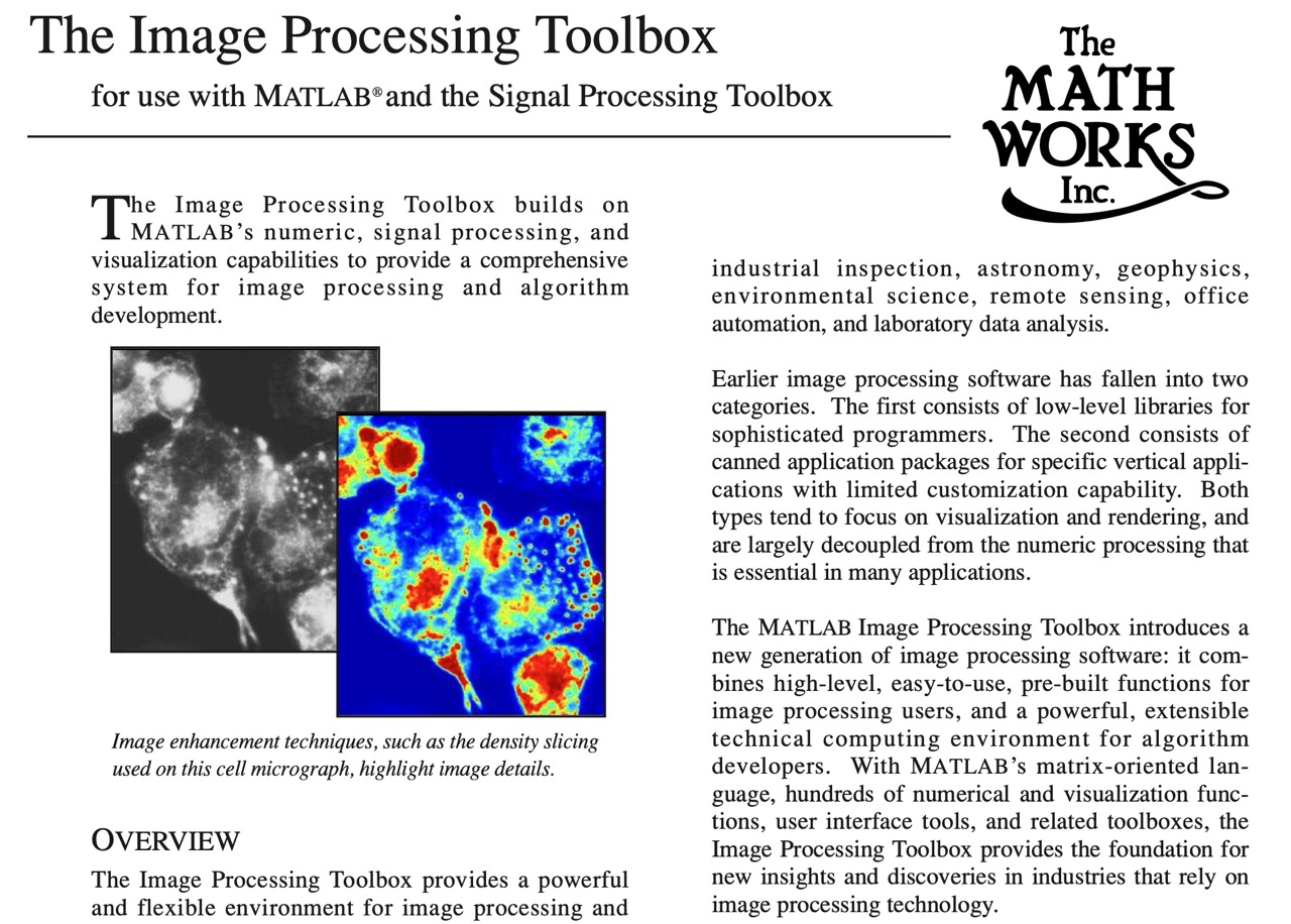
Excerpt from Image Processing Toolbox v1 datasheet, 1993
For the purpose of this series on the history of MATLAB image display, I’ll zoom in to view one function in detail: imshow.
The Function IMSHOW and Image Types
Here is the help text for the v1.0 implementation of imshow:
%IMSHOW    Display image data.
%    IMSHOW is used to display all types of images: indexed images,
%    intensity images, and RGB images.
%
%    IMSHOW(X,MAP) displays the indexed image A with the colormap MAP.
%    IMSHOW(I,N) displays the intensity image I with a gray scale
%    colormap of length N.
%    IMSHOW(R,G,B) displays the RGB image in the intensity matrices
%    R,G,B with an approximate colormap based on uniform quantization.
%
%    IMSHOW(A) looks at the data in the matrix A to determine the
%    type of image (see ISIND, ISBW, and ISGRAY) and displays the result
%    with the current colormap.  If A isn't one of the image types, it
%    is displayed using IMAGESC.
%
%    IMSHOW(x,y,A,...) uses the vectors x,y to define the axis
%    coordinates.
%
%    H = IMSHOW(...) returns a handle to the created image object.
%
%    See also IMAGE, IMAGESC.
The first sentence of the help text highlights a critical aspect of the Image Processing Toolbox design—the different image types. I mentioned in the previous series post that image display in MATLAB 4 only supported one image display model, the indexed image. By image display model, or image type, I mean the different ways that a value in a matrix can represent a particular color.
Indexed Images
I mentioned indexed images briefly in part 2. With an indexed image, the color of each displayed image pixel is determined by using that pixel value as an index into the colormap. Image Processing Toolbox version 1.0 included an indexed image called trees that was used widely in product examples at that time.
load trees X map
imshow(X,map)
title("Indexed Image Display Model")

The index matrix, X, contains positive integers that are used to index into the colormap matrix, map, to determine the colors of the corresponding image pixels.
idx = X(115,92)
idx = 19
map(idx,:)
ans = 1x3

0.6471    0.1294    0.0627
Here’s the color of the single pixel corresponding to X(115,92):
imshow(X(115,92),map)

The indexed image display model was directly supported by the MATLAB Handle Graphics image object of MATLAB 4.
Grayscale Images
Image Processing Toolbox v1 also supported the grayscale image display model. A grayscale image was represented in the toolbox by a matrix containing values ranging from 0 to 1. The value 0 corresponded to black; the value 1 corresponded to white; and values in between corresponded to shades of gray.
Note that the $[0,1]$ convention is mathematical in spirit. The convention works well with mathematical operators and color science formulas, but it was different from what many image processing researchers expected, which was a $[0,255]$ convention that was based on the range of 8-bit unsigned integers. But that didn’t make sense for MATLAB and the Image Processing Toolbox at the time, because MATLAB matrices were all floating point; there were no other numeric types in MATLAB until MATLAB 5 in 1997.
For many years, toolbox documentation used the variable name I for grayscale images. That’s because these were called intensity images in early toolbox versions.
I = ind2gray(X,map);
I(100:105,180:185)
ans = 6x6

0.0592    0.2142    0.0592    0.2142    0.1789    0.2142
0.0592    0.2142    0.0592    0.0592    0.2142    0.0592
0.0592    0.0592    0.2142    0.2142    0.0592    0.2483
0.2142    0.2142    0.0592    0.0592    0.2142    0.0592
0.2142    0.0592    0.2142    0.0592    0.2142    0.2142
0.2142    0.0592    0.2142    0.0592    0.1789    0.0592
imshow(I)
title("Grayscale Image Display Model")

Binary Images
Image Processing Toolbox version 1 included the concept of binary images, but this model was not clearly distinguished from grayscale images at the time. A binary image was represented by a matrix containing only 0s and 1s. Comparing with the grayscale model, you can see that a binary image was just a grayscale image that happened to contain only 0s and 1s. If you passed a matrix to a function that expected a binary image input, such as bwperim, the function would force the input to have only 0s and 1s using code like this:
im = im ~= 0;
The help text for imshow didn’t even mention binary images. That is probably because the code for displaying a grayscale image worked just fine for displaying a binary image.
Early toolbox documentation commonly used BW as the variable name in examples about binary images.
BW = imbinarize(ind2gray(X,map));
imshow(BW)
title("Binary image display model")

Truecolor Images
The term truecolor image was widely used in the 1990s to refer to an image whose pixels are represented using three 8-bit numbers—one for the red component, one for the green component, and one for the blue component. When talking about a computer’s graphics capabilities, this was often called 24-bit color.
Since MATLAB did not yet have multidimensional arrays, Image Processing Toolbox version 1 was designed to represent truecolor images with three matrices, each with values ranging from 0 to 1, just like the grayscale image convention. Toolbox documentation typically used the variable names R, G, and B for these three matrices.
Today’s Image Processing Toolbox does not support the three-matrix representation, but I can show you what the matrices would have looked like with the following code:
[R,G,B] = imsplit(ind2rgb(X,map));
R(100:102,200:202)
ans = 3x3

0.0627    0.1922    0.1922
0.1922    0.2588    0.1922
0.1922    0.0941    0.0627
G(100:102,200:202)
ans = 3x3

0.0627    0.2235    0.2235
0.2235    0.1608    0.2235
0.2235    0.2588    0.0627
B(100:102,200:202)
ans = 3x3

0.0314    0.2235    0.2235
0.2235    0.0627    0.2235
0.2235    0.0314    0.0314
tiledlayout("flow")
nexttile
imshow(R)
title("Red component")
nexttile
imshow(G)
title("Green component")
nexttile
imshow(B)
title("Blue component")

In 1993, the syntax imshow(R,G,B) would have been used to display this truecolor image.
Limitations of 1993 Image Display
There were several significant limitations of the MATLAB 4 + Image Processing Toolbox 1 + imshow image display solution. The limitations were generally related to display speed, loss of original pixel values in the image object, and display quality.
Display Speed
I don’t have any way to run comparison benchmarks for you today, in 2025, but our 1993 MATLAB users loudly complained that image display speed was slow, slow, slow. There were a few contributing factors:
- Slow MATLAB graphics rendering
- An toolbox design that caused computational slow-downs on most function calls
- The image type conversion required because of the limited MATLAB image display model
MATLAB 4 Handle Graphics was indeed a huge step forward in the early 1990s, but it was no speed demon. Big improvements would come later, in 1997, with the arrival in MATLAB of both faster software rendering (via zbuffer and double buffering) and hardware-accelerated rendering (via OpenGL).
The toolbox design quirk that slowed things down was the need, for most toolbox functions, to do a data-dependent determination of the image type. This involved a time-consuming pass over every pixel (matrix element) to see if they were all positive integers, or if they were all values between 0 and 1, or if they were only the values 0 and 1. A substantial toolbox redesign solved this particular problem in 1997.
As for the image type conversion, remember that MATLAB 4 image display was limited to the indexed image model. How, then, did imshow display a truecolor image? The function imshow displayed such an image by converting it, on-the-fly, using color quantization and color dithering, to an indexed image with only 216 colors. (Go ahead, read that sentence again.) Here is the relevant piece of imshow code from back then:
[mp1 mp2 mp3] = meshgrid(0:.2:1,0:.2:1,0:.2:1);
map = [mp1(:) mp2(:) mp3(:)];
c = dither(arg1,arg2,arg3,map); % Uniform quantization, max. 216 colors
That was a lot of computational work that had to be performed before any image pixel color could hit the screen.
Loss of Original Pixel Values
Perhaps this one is more about programming with the image object rather than display. The image object has a property called CData, and this property contains all the image pixel values. In 1993, this property had the form of a two-dimensional matrix. (Today, it might also have the form of an $M\times N\times 3$ array.
Because of the image type conversion, though, the image CData property did not contain the original pixel values that were provided by the imshow caller. Those original pixel values had undergone a mathematical transformation, either scaling and rounding, or quantization and dithering, to become positive integer index values.
I think the drawbacks did not become apparent until the experiments in the mid-1990s with developing an image processing GUI of some kind, using MATLAB Handle Graphics. We realized that if, for example, we wanted to display the pixel values, or perhaps statistics about the pixel values (mean, median, range, etc.), we wouldn’t be able to get the original pixel values from the image object embedded within the GUI. We could work around that, but only by making things slower and more memory-intensive.
Display Quality
Image display quality was affected by two factors, one of which was really independent of MATLAB—the limited number of colors in typical computer monitors at the time. Most of the graphics cards MATLAB users had in 1993 could only display 256 colors at once. And that included system and user interface colors, like windows, menus, dialog boxes, etc. For this reason, the default colormap length in MATLAB back then, and for many years after, was 64.
The following code simulates what a grayscale ramp image might have looked like when displayed using imshow and MATLAB 4 on most computers at the time.
clf
ramp = repmat(linspace(0,1,600),300,1);
imshow(ramp)
colormap(gray(64))

If you look closely, you can see the vertical bands. These are caused by the quantization of the image display into only 64 distinct levels of gray.
When displaying a truecolor image, which theoretically could have as many as $2^{24} \approx 17$ million colors, the function imshow displayed it using color dithering and only 216 distinct colors. Consider the first image below, which is a screen capture of a modern MATLAB graphic display. The second image is a zoomed-in view of the first. The third image is the same zoomed-in view, but of an indexed image created using color dithering, as imshow would have shown in 1993.
clf
tiledlayout
nexttile
imshow("surf-peaks.png")
title("Original")

nexttile
imshow("surf-peaks.png")
xlim([245 304])
ylim([557 599])
title("Zoomed in")

nexttile
imshow("surf-peaks-dithered.png")
xlim([245 304])
ylim([557 599])
title("Dithered to 216 colors")

The other factor explains why the first image below might have looked like the second image below when displayed using the 1993 version of imshow.


The quality problem was related to the size of the image as displayed on the screen. This issue was addressed by later changes in imshow, but those changes caused a lot of other problems and turned out to be fragile.
It is a complicated issue, and I hope to explain it fully in the next post in this series.